Wednesday, June 4, 2014

Necessity and availability of number formats in Cell Format feature

Excel’s custom number formatting is very important yet probably the most underutilized feature.  Understanding and mastering this feature can greatly enhance the visual design of your Excel workbooks.  The key benefit of custom number formatting is that it allows you to change the appearance of your data without actually changing the data value behind the appearance. A number format does not affect the actual cell value that Microsoft Excel uses to perform calculations. The actual value is displayed in the formula bar, which is the bar at the top of the Excel window that you use to enter or edit values or formulas in cells or charts that displays the constant value or formula stored in the active cell.


Now for one who doesn’t have understand the custom number formatting will often go through the process of changing their data values rather than just the presentation of those values. For example, consider a user who wants to show 1,000,000 as 1.0 M.  Instead of using formatting, the user decides to divide his value by 1,000,000 and concatenates an “M” to the end of it.  In doing so, not only does he add an additional step in his model, but such a step is also rarely documented, which can create confusion if the work needs to be handed off to another person. Moreover, if he or she has to use this number, the concatenated 1.0 M will not suffice since it now contains a text formula. An even worse case if is the user decides to remove the link between the display value and the actual value altogether.  He or she simply hardcodes the value by typing in 1.0 M.  At that point, any changes made to the original 1,000,000 value will not translate through to what is displayed. 

Number formats that are available on the Number ribbon of the Home main tab. By clicking on Number ribbon, a dialog box named Format Cells will open.


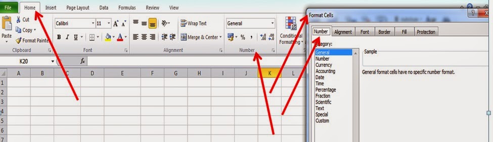
The formatting options are available if one clicks on the Number section.

General
This is the default number format that Excel applies when you type a number, which means it does not have any special formatting rules. For the most part, numbers that are formatted with the General format are displayed just the way you type them. However, if the cell is not wide enough to show the entire number, the General format rounds the numbers with decimals. The General number format also uses scientific (exponential) notation for large numbers (12 or more digits). This means when you enter data in a cell, Excel tries to guess what format it should have. When it doesn’t guess correctly, you need to change the format. 

Number
This format is used for the general display of numbers. You can specify the number of decimal places that you want to use, whether you want to use a thousand separator (such as 1,234 instead of only 1234) and how you want to display negative numbers.

Currency
This format is used for general monetary values and displays the default currency symbol with numbers. You can specify the number of decimal places that you want to use, whether you want to use a thousand separator, and how you want to display negative numbers.

Accounting
This format is also used for monetary values, but it aligns the currency symbols and decimal points of numbers in a column.

Date
This format displays date and time serial numbers as date values, according to the type and locale (location) that you specify. Except for items that have an asterisk (*) in the Type list (Number tab, Format Cells dialog box), date formats that you apply do not switch date orders with the operating system.

Time
This format displays date and time serial numbers as time values, according to the type and locale (location) that you specify. Except for items that have an asterisk (*) in the Type list (Number tab, Format Cells dialog box), time formats that you apply do not switch time orders with the operating system.

Percentage
This format multiplies the cell value by 100 and displays the result with a percent symbol (%). You can specify the number of decimal places that you want to use.

Fraction
This format display a number as a fraction, according to the type of fraction that you specify.

Scientific
This format displays a number in exponential notation, replacing part of the number with E+n, where E (which stands for Exponent) multiplies the preceding number by 10 to the nth power. For example, a 2-decimal Scientific format displays 12345678901 as 1.23E+10, which is 1.23 times 10 to the 10th power. You can specify the number of decimal places that you want to use.

Text
This format treats the content of a cell as text and displays the content exactly as you type it, even when numbers are typed.

Special
This format displays a number as a postal code (ZIP Code), phone number, or Social Security number.

Custom
This format allows you to modify a copy of an existing number format code. This creates a custom number format that is added to the list of number format codes. You can add between 200 and 250 custom number formats, depending on the language version of Excel that you have installed.


Thursday, May 29, 2014

Paste Special Live Preview in Excel 2010

If you right-click a range of cells and select Paste Special, Excel 2010 brings up a live preview of the possible menu choices, as shown below.


Clicking an option lets you see a preview of how your spreadsheet will appear if you choose that option.


The short cut key for paste special Alt + E + S. Doing so, the paste Special window will open.


As you can see, the short cut key for each option is given as underlined character. For example, Paste Special-Formats has underlined "t". Hence, if you want to paste format only, you have to go for Alt+E+S+T. Similar procedures must be followed for other paste special options.


Wednesday, May 28, 2014

Improved Data Bars in Excel 2010

Excel 2007 introduced using data bars as a method to summarize numerical data. In Excel
2010 data bars have been improved in two ways: 
  • You can choose either Solid Fill or Gradient Fill for shading.
  • Data bars recognize negative numbers.

 
Figure given above shows an example of how the new data bars appear. Rows 4-11 contain gradient shading, and rows 1217 contain solid shading.

I will discuss this feature in details later when I will cover conditional formatting.

Sunday, May 25, 2014

New Equation Editor in Excel 2010

In Excel 2010 you can create equations in Excel. If you select Insert from the ribbon, you can then click Equation at the far right to bring up the equation templates as shown below.


For example, if you want to type an equation involving a summation sign, choose one of the Large Operator options.


Sometimes you want a well-known equation (such as the quadratic formula) to appear in your spreadsheet. After choosing Insert, click the drop-down arrow to the right of Equation to import an already completed equation (such as the quadratic formula). Of course, after choosing Insert you select Symbol, you can insert mathematical symbols (such as the Greek letter μ) into a cell.


Sunday, May 18, 2014

File Tab in Excel 2010

Excel 2007 introduced the Office button. In Excel 2010, the Office button has been replaced by the File tab. The File tab is located at the left end of the ribbon. After selecting File, you are presented with the choices as shown below.


You can see that the File tab combines the Print and File menus from previous versions of Excel. Also, selecting Options lets you perform a variety of tasks, such as customizing the ribbon or the Quick Access Toolbar, or installing add-ins. In Excel 2007 these tasks (except for customizing the ribbon) were performed after clicking the Office button.

Saturday, May 17, 2014

Customizable ribbon in in Excel 2010

The Ribbon is the strip of buttons and icons located above the work area introduced with Excel 2007 that replaces the menus and toolbars found in earlier versions of Excel. Above the Ribbon are a number of tabs, such as Home, Insert, and Page Layout. Clicking on a tab displays the options located in this section of the ribbon. When any file opens, the options under the Home tab are displayed, which are grouped according to their function - such as Clipboard (includes cut, copy, and paste options), and Font (includes current font, font size, bold, italic, and underline options).


Clicking on an option on the ribbon may lead to further options contained in a Contextual Menu or dialog box that relate specifically to the option chosen. However, in Excel 2007, users were not able to customize the tabs displayed across the top of the ribbon. In Excel 2010, it is easy to customize the appearance of the ribbon tabs. Begin by selecting File in the upper-left portion of the ribbon. After choosing Options, you’ll see the Customize Ribbon page as shown below.


Now, if you want to show a new tab, say Developer. For that, simply select Developer in the list at the right, and click OK. You could also deselect in the same way. This video tutorial could help you understand.


You can change the order in which the tabs appear by selecting a tab, and then using the Move Up and Move Down arrows on the right.


If you click the drop-down arrow by Main Tabs, you can display Tool tabs. Then you can customize the tabs that appear when a given object is selected. For example, if you clear Format under Chart Tools, when you select a Chart object, the Format tab does not appear.


Clicking the New Tab button allows you to create a new tab, and the New Group button lets you create a group within a tab. Of course, you can use the Rename button to change the name of a group or tab.


The Quick Access Toolbar is an old function from Excel 2007 that can still be very useful. You probably use some Excel commands much more often than others. Having to switch between tabs to find the command you need might slow you down. The Quick Access Toolbar allows you to collect your favorite commands in one place. The default location of the Quick Access Toolbar is above the ribbon in the upper-left portion of the Excel window.


You can add a command to the Quick Access Toolbar simply by right-clicking the command and choosing Add To Quick Access Toolbar. You can also add commands by clicking File in the upper-left portion of the ribbon. Next click Options, and then display the Customize the Quick Access Toolbar page. After choosing a command you want to add, select Add, and click OK. Of course, the Move Up and Move Down arrows let you customize the order in which icons appear. You can remove any command from the Quick Access Toolbar by right-clicking the command, and then clicking Remove From Quick Access Toolbar. You can move the Quick Access Toolbar below the ribbon by right-clicking the toolbar, and selecting Show Below The Ribbon.


People sometimes have trouble finding commands that appeared in earlier versions of Excel that seem to have disappeared from Excel 2010. For example, you might be a fan of the old method used to create PivotTables. If you still want to use the layout method, you can find it by clicking the drop-down arrow to the right of Popular Commands and choosing Commands Not In The Ribbon. After scrolling down (pressing the P key several times is probably quicker!), you will find the PivotTable And PivotChart Wizard command, which you can then add to your Quick Access Toolbar.


Friday, May 16, 2014

What’s New in Excel 2010

Microsoft Excel 2010 contains many new features that are very helpful for carrying out various activities:

Customizable ribbon: Now you can completely customize the appearance of the ribbon.

Sparklines: Cool graphs that summarize lots of data in a single cell.

Slicers: Dashboard controls that make “slicing and dicing” PivotTable calculations much easier.

PowerPivot: A free add-in that enables you to quickly create PivotTables with up to
100 million rows of data based on data from many sources (databases, spreadsheets, and websites).

Solver: An improved Solver allows you to find the “best” solution to many business problems for which previous versions of the Solver returned incorrect answers.

File tab: The new File tab on the ribbon replaces the Office button and allows easy access to the File and Print menus.

Updated statistical functions: The accuracy of Excel statistical functions has been improved, and several new functions (including RANK.EX, AGGREGATE, WORKDAY.INTL, and NETWORKDAYS.INTL) have been added.

Equations: You can now edit equations in Excel by using an equation editor that is similar to the Microsoft Word equation editor.

Data bars: Data bars have been improved.

Paste Special: Paste Special options now include a live preview.


All the features will be discussed later in details in the following posts. Keep reading !!!!